WFSS

Summary

The WFSS observing mode enables multi-plex, low-resolution spectroscopy (R=150) over most of the 2.2’x2.2′ field of view. A choice between two grisms, one dispersing along detector rows, the other along columns, is available to mitigate contamination in crowded fields. The wavelength coverage is bound between 0.8 and 2.3 microns, as selected through the use of a blocking filter (F090W, F115W, F140M, F150W, F158M, F200W). WFSS is particularly well suited to detect emission lines in spectra of high-redshift galaxies when conducting deep-field surveys. But other science projects (identifying low-mass objects in star-forming regions) can also be tackled.

Operations Concept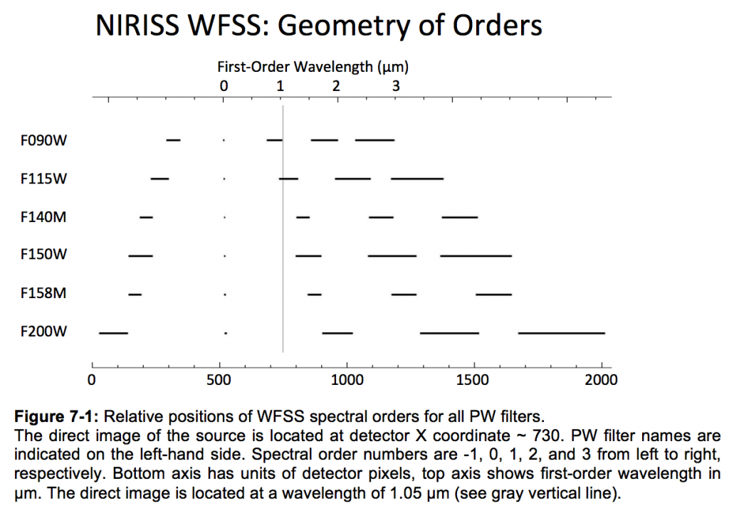

To allow precise wavelength calibration as well as better identify sources in a field, a direct image (without grism) is acquired both before and after a set of dithered exposures through a grism. Direct images are taken through the same blocking filter as the grism sequence. There is a choice for the number of dither positions used in the sequence  (between 2 and 8 positions). If observations make use of two grisms or more than one filter, before/after direct images are obtained for each grism and/or each filter setting.

The grisms undeviated wavelength is 1.05 microns which means that direct images and grism images are aligned only at that precise wavelength. First order wavelengths in the grism images are systematically deviated by several tens (F090W, F115W) to a few hundreds of pixels (F140M, F150W, F158M, F200W), see figure above (courtesy STScI). In other words, a source found near the edge of the detector in a direct image may have its spectrum out of the field of view. The effective field of view in the WFSS mode is therefore slightly smaller than in the Imaging mode.

Contamination

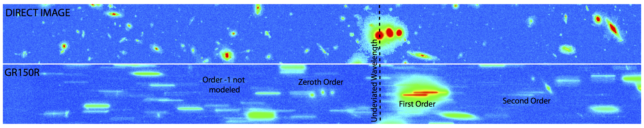
Below is an image slice (2048×200 pixels) of a simulation of the lensing cluster MACS0416 observed with NIRISS in the WFSS mode (courtesy Chris Willott). The dispersed image shows spectral traces of different objects often overlapping. In addition, the first order spectrum is contaminated by other diffraction orders (0th, 2nd, -1 not modeled). Most of the contamination degeneracies can be lifted by duplicating observations with the GR150 dispersing in the other direction. To extract information optimally in this case, a model of each source needs to be generated and subtracted from the observation, in an iterative approach. For less crowded fields, contamination is less of a problem.

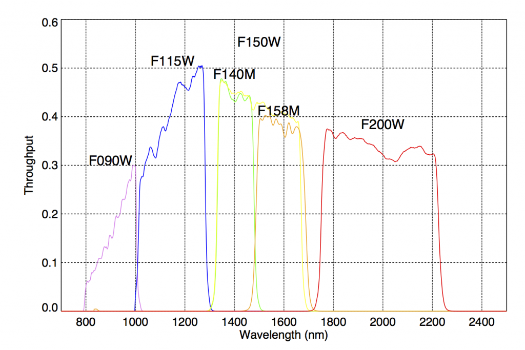
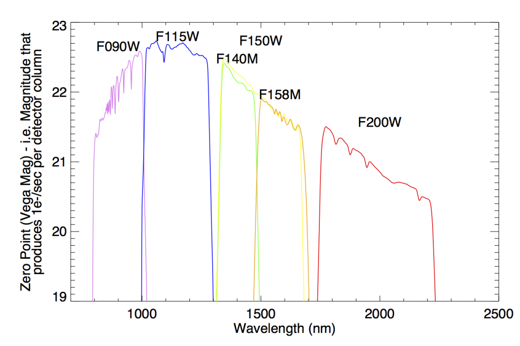
Throughput and Zero Points

The blaze function of GR150 grisms peak at ~1.2 microns in first order with a transmission better than 80%. The total system throughput (telescope + instrument + detector + grism + filter) is shown  below. The absolute total throughput is shown at left. At right, the throughput is expressed as zero points.

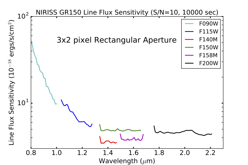
Sensitivities

Assuming a line-emission spectrum, the WFSS sensitivity at 10 sigma was computed for a wall clock time of 10000 sec split into 10 integrations of 1000 sec. Various parameters feed into this plot:

• The assumed throughput is the as-measured throughput reduced by its 1-sigma uncertainty (19%). The following uncertainties add up in quadrature to 19%: Filter transmission (5%), Encircled energy in the PSF (5%),  Optical train reflectivity (2% per each of the 7 surfaces), Grism blaze function (10%), Detector quantum efficiency (15%).
• The background signal is 1.2X that estimated by Jane Rigby (see below) which includes zodiacal light, instrument emission (negligeable at the WFSS wavelengths) and scattered light.
• The cosmic ray hits have the effect of reducing the effective integration time by 20% over an integration of 1000 sec.
• The ensquared PSF energy within the 3×2 aperture encompasses 72-78% of the total astrophysical flux, depending on wavelength.
• The readout noise (see below) is parametrized as: noise = sqrt(Tint*dc+(58*Tint^-0.344)^2) which includes the dark current assumed to be 0.0382 e-/sec.

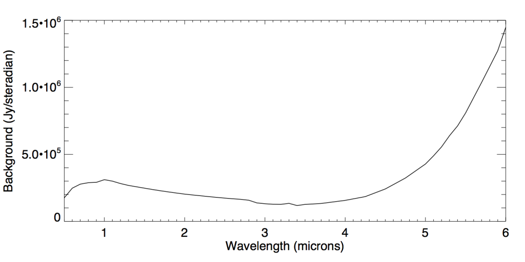
Background Noise

This model was computed by Jane Rigby. It includes zodiacal light, instrument emission and scattered light.

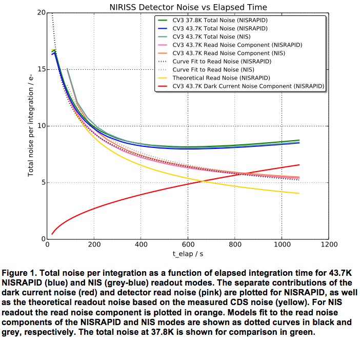
Readout Noise

For deep field observations, an important noise component  is the detector readout noise. One would expect the readout noise in a integration to decrease as sqrt(1/Ngroup) where Ngroup is the number of non-destructive reads in an integration. An analysis carried by Chris Willott on actual images indicate that a readout noise plateau is reached at Ngroup ~ 50. In the figure below, time elapsed can roughly be converted to Ngroup by dividing by 10.